
MATLAB in Perception Classes – Introductory Exercises
1 August 2026
MATLAB has become an important tool in scientific research and, for this reason, its early introduction within a university degree programme is desirable. Moreover, in the specific context of teaching Psychology of Perception (although certainly not exclusively), it enables students to actively engage with basic principles at a level that would be difficult to achieve using traditional pedagogical strategies.
On the other hand, given the entry requirements for a degree in Psychology (at least in the Portuguese context), one would not expect a typical student to possess sufficient programming skills for immediatelly adapting to the MATLAB environment or, at the very least, for it to be easily accessible. Far from constituting an insurmountable obstacle, this merely suggests that the use of MATLAB should prioritise a clear connection with the course content, relegating a comprehensive understanding of its programming syntax to a secondary role, even if this entails sacrificing some computational efficiency in favour of greater procedural transparency.
The following exercises constitute the students’ first encounter with MATLAB in my classes and are included within the introductory topics on Vision and Colour Perception. Consequently, the first exercise provides an interactive illustration of elementary principles of additive colour mixing (based on the light emitted by the screen; a brief prior explanation of the underlying hardware is recommended) and enables students to grasp the concept of metameric colours, as well as certain aspects of the Helmholtz–Young Theory (or Trichromatic Theory). The second and third exercises expand upon these concepts through the use of photographs (to encourage greater engagement, students may be invited to use photographs of themselves). These exercises were adapted from those proposed in Chapter 8 of Wallisch et al. (2014), although they have been considerably simplified to increase their pedagogical accessibility. They may be completed by students, either with or without supervision, or adapted into a script (simply by copying and pasting all the commands below into a new script and, after saving the file, running it) to be used in class by the lecturer, the students, or both. This latter option has the advantage of taking up less class time, although at the cost of reducing students’ direct engagement with MATLAB.
Preliminary Requirement
Exercises 2 and 3 require the ‘Image Processing Toolbox’ add-on, which can be easily installed through MATLAB’s Add-On Explorer. This add-on is particularly useful for MATLAB-based exercises in a course covering topics related to perception.
Exercise 1 – The RGB System and Additive Colour Mixing
Begin by running the following commands in the MATLAB Command Window. These simply assign values to three variables (R, G, and B). In this case, the values represent, in bytes, the intensity of each of the three channels in the RGB system (R = red; G = green; B = blue). The specific values can – and should – be varied. A value of 127 in all three channels will produce a medium grey; equal values in all three channels that are higher or lower than 127 will produce lighter or darker greys, respectively; values of 0 or 255 in all three channels will produce white or black, respectively; finally, different values across the three channels will produce any possible colour hue (independent experimentation, by running this exercise several times, should be strongly encouraged here).
R = 127;     % Value of the red ([R]ed) channel, in bytes (between 0 and 255)
G = 127;     % Value of the green ([G]reen) channel, in bytes (between 0 and 255)
B = 127;     % Value of the blue ([B]lue) channel, in bytes (between 0 and 255)
Once the values of the R, G, and B channels have been defined, they must now be combined within the same area of the screen. To do this, begin by defining a 3 (horizontal dimension) × 3 (vertical dimension) × 3 (number of channels) matrix, initially containing only 0s:
matrix = zeros(3,3,3); % Create a 3 × 3 × 3 matrix containing 0s
For this matrix to be correctly interpreted as RGB values, it must be converted to uint8 (8-bit unsigned integer arrays):
matrix = uint8(matrix); % Convert the matrix to uint8
The R, G, and B values must now be assigned to the corresponding channels of this matrix (that is, to its third dimension). To ensure that the resulting colour can be easily distinguished, these values will be assigned only to the central position in the horizontal and vertical dimensions (the remaining cells, arranged around this central cell, will retain a value of 0 and will therefore produce a black surrounding area):
matrix(2,2,1) = R;     % Assign the value of the red channel (R)
matrix(2,2,2) = G;     % Assign the value of the green channel (G)
matrix(2,2,3) = B;     % Assign the value of the blue channel (B)
Finally, to display the result, simply run the following command:
image(matrix) % Display the matrix as an image
As mentioned above, the entire exercise can and should be repeated using different values for R, G, and B.
Exercise 2 – Separating the RGB Channels of a Digital Photograph
Begin by reading and importing a digital image into the MATLAB environment as a matrix. In the following command, replace “name” with the name of the file (which should be placed in MATLAB’s current folder) and “extension” with the file-type extension (e.g. jpg, png):
Photo = imread('name.extension'); % Import an image as a matrix
Since each channel (R, G, and B) of the original image will be isolated, matrices capable of storing the corresponding values must first be created. To do this, create three new matrices – one for each RGB channel – with the same horizontal and vertical dimensions as the original image and initially containing only 0s:
ChannelR = zeros(size(Photo,1),size(Photo,2),3);     % Create the ChannelR matrix with the same horizontal and vertical dimensions as the Photo matrix
ChannelG = zeros(size(Photo,1),size(Photo,2),3);     % Create the ChannelG matrix with the same horizontal and vertical dimensions as the Photo matrix
ChannelB = zeros(size(Photo,1),size(Photo,2),3);     % Create the ChannelB matrix with the same horizontal and vertical dimensions as the Photo matrix
Each of the three RGB channels of the original image can now be copied into its corresponding matrix (which must also be converted to uint8):
ChannelR(:,:,1) = Photo(:,:,1);     % Copy the values from the first layer of the third dimension (the R channel) of the photograph into the corresponding layer of the ChannelR matrix
ChannelR = uint8(ChannelR);     % Convert to uint8

ChannelG(:,:,2) = Photo(:,:,2);     % Copy the values from the second layer of the third dimension (the G channel) of the photograph into the corresponding layer of the ChannelG matrix
ChannelG = uint8(ChannelG);     % Convert to uint8

ChannelB(:,:,3) = Photo(:,:,3);     % Copy the values from the third layer of the third dimension (the B channel) of the photograph into the corresponding layer of the ChannelB matrix
ChannelB = uint8(ChannelB);     % Convert to uint8
Finally, to display both the original image and each of its constituent channels – red [R], green [G], and blue [B] – the subplot function can be used:
figure;     % Open figure
subplot(2,2,1);     % In a 2 × 2 grid of panels, select the first panel
image(Photo)     % Display the original photograph in the selected panel
subplot(2,2,2);     % In a 2 × 2 grid of panels, select the second panel
image(ChannelR)     % Display the ChannelR matrix in the selected panel
subplot(2,2,3);     % In a 2 × 2 grid of panels, select the third panel
image(ChannelG)     % Display the ChannelG matrix in the selected panel
subplot(2,2,4);     % In a 2 × 2 grid of panels, select the fourth panel
image(ChannelB)     % Display the ChannelB matrix in the selected panel
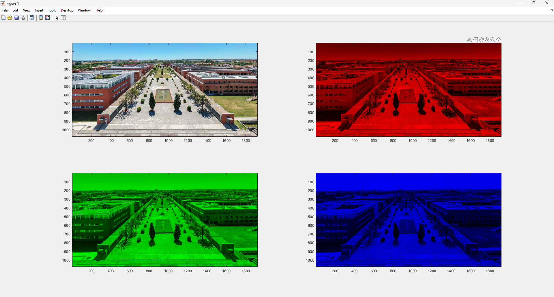
The result should resemble Figure 1.
Exercise 3 – Removing Each of the Three RGB Channels from a Digital Photograph
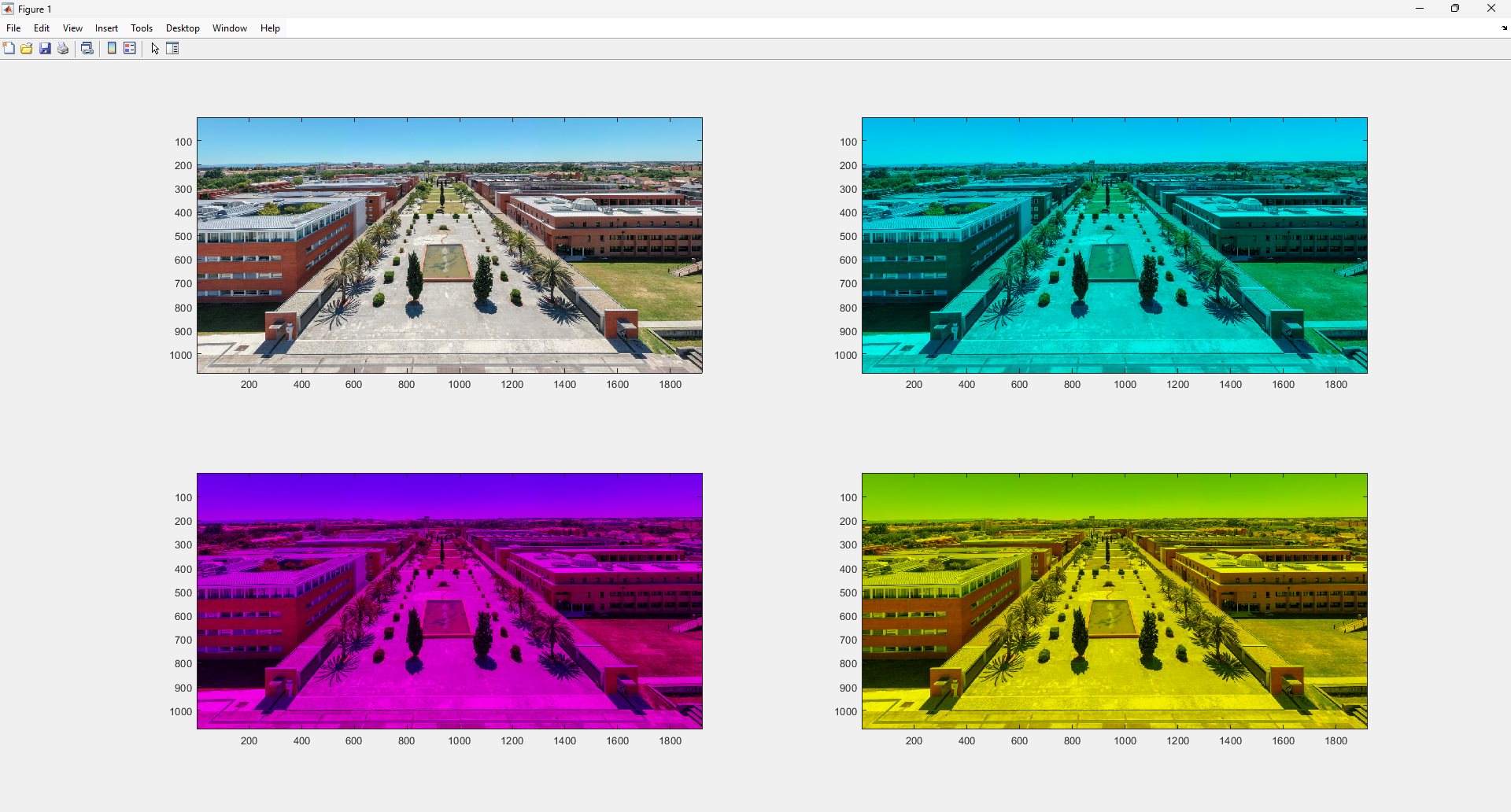
In a sense, this exercise complements the previous one. Rather than isolating each RGB channel, the channels will be selectively removed from the original photograph. The result will be three new images: one without the red channel (containing only the green and blue channels), another without the green channel (containing only the red and blue channels), and a third without the blue channel (containing only the red and green channels).
An interesting aspect of this exercise is that it simulates what might be expected from the different types of dichromacy (protanopia, deuteranopia, and tritanopia) solely on the basis of the Helmholtz–Young Theory. It is important to emphasise that, in reality, dichromacy does not resemble the result of this exercise (a simulation of colour perception in dichromacy, albeit a crude one, can be found in this other tutorial). These observations provide an important basis for linking the present exercises more directly to the course content of a perception module and may serve as a useful starting point for a formal presentation of Ewald Hering’s Opponent-Process Theory.
uma simulação da percepção das cores nas dicromacias é o alvo neste outro tutorial
Thus, as in the previous exercise, begin by importing any image (once again, replace the terms “name” and “extension” with the name and extension of the digital photography). In addition, create a matrix containing only 0s and having the same dimensions as the imported photograph:
Photo = imread('name.extension');     % Import an image as a matrix
Zeros = zeros(size(Photo,1),size(Photo,2),3);     % Create the Zeros matrix with the same dimensions as the original photograph
Next, for each case in which one of the channels (R, G, or B) is excluded, generate a corresponding matrix. Initially, this matrix will simply be a copy of the original photograph. In the next step, the channel to be excluded is replaced by its equivalent from the Zeros matrix. Finally, each of these matrices is converted to uint8:
% Image WITHOUT the red (R) channel:
xGB = Photo;
xGB(:,:,1) = Zeros(:,:,1);
xGB = uint8(xGB);

% Image WITHOUT the green (G) channel:
RxB = Photo;
RxB(:,:,2) = Zeros(:,:,2);
RxB = uint8(RxB);

% Image WITHOUT the blue (B) channel:
RGx = Photo;
RGx(:,:,3) = Zeros(:,:,3);
RGx = uint8(RGx);
Lastly, as in Exercise 2, the results are displayed in a 2 × 2 grid of panels:
figure;
subplot(2,2,1);
image(Photo)
subplot(2,2,2);
image(xGB)
subplot(2,2,3);
image(RxB)
subplot(2,2,4);
image(RGx)
The final result should be similar to that shown in Figure 2.
Biliography
- Wallisch, P., Lusignam, M. E., Benayoun, M. D., Baker, T. I., Dickey, A. S., & Hatsopoulos, N. G. (2014). MATLAB for Neuroscientists: An Introduction to Scientific Computing in MATLAB (2nd Ed.). Elsevier Academic Press.