Fitting psychometric functions

Fitting psychometric functions with Microsoft Excel

6 August 2026

Psychometric functions are an important tool in Classical Psychophysics (or Local Psychophysics). Commonly associated with the Method of Constant Stimuli, or related variants, they describe the relationship between the proportion of a given comparative judgement (e.g. greater/smaller, more intense/less intense, etc.) and the intensity of a set of stimuli – the Comparison Stimuli – relative to a reference stimulus – the Standard Stimulus. Once their parameters have been estimated from empirical data, psychometric functions make it possible to determine the Point of Subjective Equality and the Difference Threshold, quantities that are fundamental for characterising a wide range of perceptual phenomena and testing theoretical hypotheses.

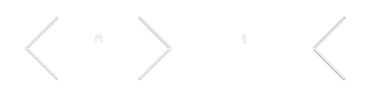
To illustrate this with a concrete example from the outset, suppose we wish to measure the magnitude of the Müller-Lyer illusion. In the version shown in Figure 1, line segments A and B are physically identical in length. Nevertheless, segment B (on the right) appears longer than segment A (on the left). This description – "appears longer" – is merely qualitative. To investigate the phenomenon scientifically, we must quantify the perceptual difference between the lengths of the two line segments. In other words, we must determine how much longer segment B appears than segment A or, equivalently, how long segment B would have to be in order to be perceived as equal to segment A (that is, the Point of Subjective Equality). In addition, we may also wish to characterise the sensitivity of length perception – that is, how much the length of segment B must change from the Point of Subjective Equality before it is perceived as longer or shorter than segment A (the Difference Threshold). Both quantities can be estimated from a psychometric function.

Figure 1. Müller–Lyer illusion. Line B is physically the same length as line A despite appearing longer.

This tutorial explains how to fit a psychometric function to a set of empirical data using Microsoft Excel. Although this is not the most sophisticated approach available for this purpose (cf. Schütt et al., 2016), it is sufficiently accurate for most applications, including many research settings. Moreover, because it relies on widely available software, it avoids the need to install and learn a specialised computational environment. Finally, since almost every step of the Least Squares fitting procedure is implemented explicitly, the method has considerable pedagogical value that would be lost if the entire procedure were carried out automatically by dedicated software.

Preliminary step – enabling the Solver add-in

Before beginning, ensure that the Solver add-in is enabled in Microsoft Excel. This feature is not enabled by default. It can be activated from the File menu by selecting Options. In the Options window, open the Add-ins section and click Go... next to Manage: Excel Add-ins. In the list of available add-ins, tick Solver Add-in and confirm by clicking OK.

Preparing the empirical data

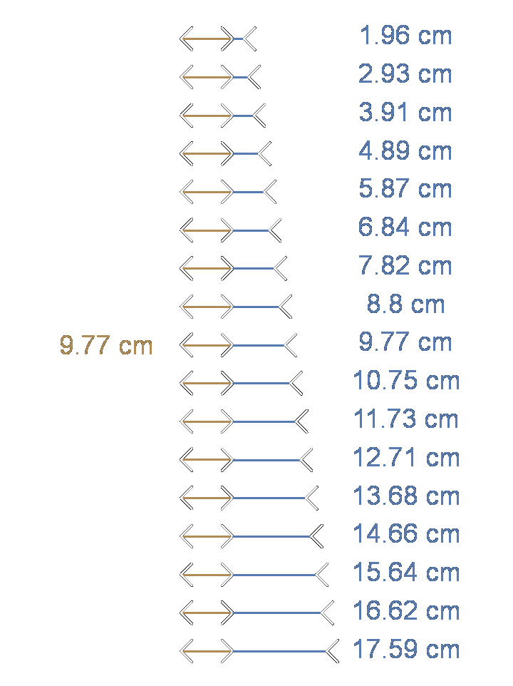
Each of the stimuli shown in Figure 2 was presented 20 times in a random order to an observer who was instructed to indicate whether the line on the right – the Comparison Stimulus – appeared LONGER or SHORTER than the line on the left – the Standard Stimulus. This is the simplest implementation of the Method of Constant Stimuli.

Müller-Lyer stimuli used to collect data with the Method of Constant Stimuli — Figure 2. Müller-Lyer stimuli used to collect data using the Method of Constant Stimuli. The values (not shown to the observer) indicate the lengths of the Standard Stimulus (left) and Comparison Stimuli (right).

The following table shows the proportion of LONGER responses for each Comparison Stimulus. Comparison Stimuli that were clearly shorter than the standard stimulus (<6.84 cm) never elicited a LONGER response. Conversely, Comparison Stimuli longer than 10.75 cm were consistently judged as LONGER, producing a proportion of 1. Between these extremes, the proportion of LONGER responses increased systematically from 0 to 1. Note that when the comparison stimulus had exactly the same physical length as the standard stimulus (9.77 cm), it was judged as LONGER on 85% of presentations. This pattern of results is typical of this type of experiment and is commonly analysed by fitting a psychometric function.

Standard Stimulus (cm)	Comparison Stimulus (cm)	Proportion of LONGER Responses
9.77	1.96	0
9.77	2.93	0
9.77	3.91	0
9.77	4.89	0
9.77	5.87	0
9.77	6.84	0.05
9.77	7.82	0.65
9.77	8.80	0.65
9.77	9.77	0.85
9.77	10.75	0.95
9.77	11.73	1
9.77	12.71	1
9.77	13.68	1
9.77	14.66	1
9.77	15.64	1
9.77	16.62	1
9.77	17.59	1

Specifying the psychometric function and its parameters

Among the many possible models for psychometric functions (see Schütt et al., 2016), we shall use the logistic function:

P_i = \frac{1}{1 + e^{-\left(\dfrac{E_c - E_{0.5}}{b}\right)}}\tag{1}

where $P_i$ denotes the estimated proportion of LONGER responses, $E_c$ the intensity of the comparison stimulus (in this example, the length of the line segment on the right in the stimuli shown in Figure 2), $E_{0.5}$ the midpoint of the psychometric function, corresponding to the Point of Subjective Equality (that is, the estimated length of the comparison stimulus that would be perceived as neither longer nor shorter than the standard stimulus, and therefore associated with a 50% probability of a LONGER response), and $b$ the slope parameter (that is, how rapidly the function rises from 0 to 1).

Since $E_{0.5}$ and $b$ are the parameters that will be estimated to maximise the fit of the function to the empirical data, we must first specify initial values for them. At this stage these values need only be reasonable approximations, as they will be refined later.

Enter the value 9.77 into cell E20 (the initial estimate for $E_{0.5}$ ; a sensible first approximation is the length of the standard stimulus) and 0.97 into cell E21 (the initial estimate for $b$ ; a reasonable choice is the spacing between successive comparison stimuli). Label column E as Psychometric Curve (cell E1) and enter the following formula into cell E2, corresponding to Equation 1 expressed using Excel syntax:

=1/(1+EXP(-((B2-E$20)/E$21)))

Notice that the reference to cell B2 changes from one row to the next, whereas the row references for E20 and E21 are fixed using the $ symbol. Copy this formula down to rows 3-18 by selecting cell E2 and dragging the fill handle in the bottom-right corner of the cell down to row 18. The final worksheet should resemble Figure 3.

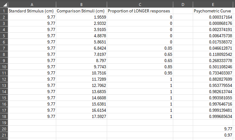
Worksheet after defining the logistic psychometric function — Figure 3. Worksheet after defining the logistic function as the psychometric function.

The values in column E represent the estimated proportions of LONGER responses produced by Equation 1 using the initial parameter estimates $E_{0.5}=9.77$ and $b=0.97$ . Although these values increase smoothly from 0 to 1, as do the empirical observations, they differ noticeably from the observed proportions. This simply indicates that the initial parameter estimates do not yet provide the best fit to the data.

At this stage you may experiment with different values for $E_{0.5}$ and $b$ (cells E20 and E21). Some values will produce estimated proportions that more closely match the observations, whereas others will produce poorer agreement. Our goal is to identify the exact parameter values that minimise the discrepancies between the observed and predicted proportions. Rather than attempting this by trial and error, we shall use the Least Squares Method, which quantifies the discrepancy between the empirical observations (column C) and the values predicted by the psychometric function (column E).

Computing the Sum of Squared Errors

To obtain a measure of the discrepancy between the empirical observations and the predictions of the psychometric function, we compute the difference between the two for each stimulus. These differences are then squared so that all values are positive and larger discrepancies contribute more heavily to the overall error.

Label column G (cell G1) as Squared Errors and enter the following formula into cell G2:

=(C2-E2)^2

Copy this formula down to cell G18 by, again, dragging down the cell.

To obtain the total error, sum all the values in column G by entering the following into cell G20:

=SUM(G2:G18)

The worksheet should now resemble Figure 4.

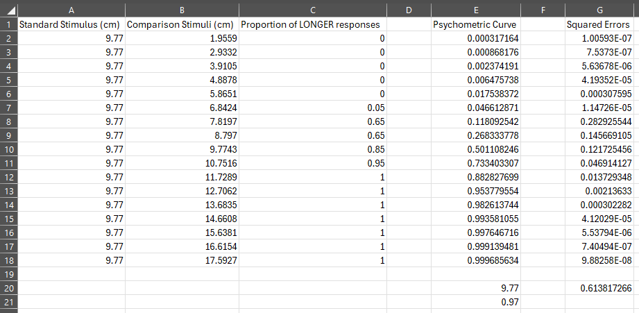
Worksheet after computing the sum of squared errors — Figure 4. Worksheet after computing the squared errors and their sum.

The value in cell G20 (the Sum of Squared Errors) measures the overall discrepancy between the psychometric function and the empirical observations. The smaller this value, the better the fit of the psychometric function to the data. Once again, you may experiment by entering different values into cells E20 and E21. You will notice that some parameter combinations reduce the Sum of Squared Errors, whereas others increase it.

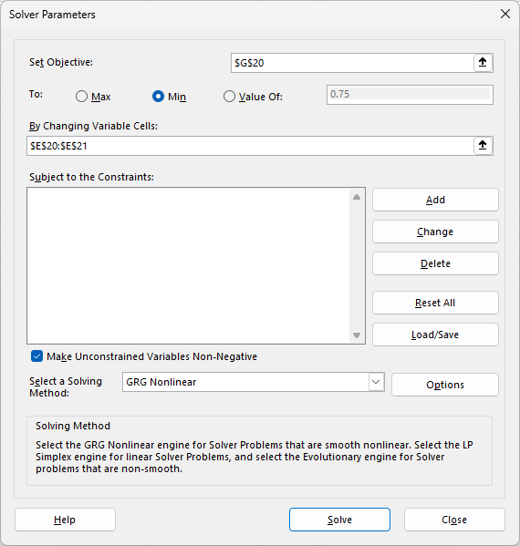
Our objective is to find the particular values of $E_{0.5}$ and $b$ that minimise the Sum of Squared Errors. To achieve this, we shall use the Solver add-in. Open it from the Data tab (typically near the upper-right corner of the ribbon). In the Solver window (Figure 5), set the Objective to cell G20, choose Min, and specify cells E20 and E21 as the By Changing Variable Cells ($E$20:$E$21; that is, the objective should be achieved by changing the values of parameters $E_{0.5}$ and $b$ ). Finally, click Solve.

Figure 5. Solver window in Microsoft Excel.

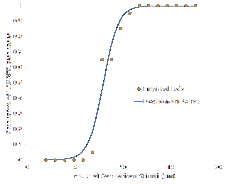
Once Solver has finished, a dialogue box summarising the optimisation results will appear. The Sum of Squared Errors (cell G20) should now be a much smaller value (typically close to zero), and cells E20 and E21 will contain the estimates of $E_{0.5}$ and $b$ that provide the best-fitting psychometric function.

To inspect the fit visually, plot the empirical proportions (column C) together with the predicted proportions (column E) in a scatter plot similar to that shown in Figure 6.

Figure 6. Observed and predicted proportions of LONGER responses as a function of comparison stimulus length.

Point of Subjective Equality and Difference Threshold

Once the psychometric function has been fitted, its parameters provide meaningful information about perceptual performance. In this example, the estimated value of the parameter $E_{0.5}$ should be approximately 7.96, corresponding to the Point of Subjective Equality. In other words, the Comparison Stimulus (the line segment on the right in Figures 1 and 2) would need to be 7.96 cm long in order to be perceived as equal in length to the Standard Stimulus (the line segment on the left). Equivalently, the line segment on the right in Figure 1 appears approximately 1.8 cm longer than the line segment on the left, despite the two being physically identical.

Determining the Difference Threshold requires one additional calculation. Because the data were collected using a two-alternative forced-choice (2AFC) task, the Difference Threshold corresponds to the comparison stimulus length associated with a predicted probability of 0.75 for a LONGER response (see Gescheider, 1997, for details). This value can be obtained by rearranging Equation 1 to solve for $E_c$ :

E_c = E_{0.5} - b\ln\left(\frac{1}{P_i}-1\right)\tag{2}

Substituting the estimated values of $E_{0.5}$ and $b$ into Equation 2, with $P_i = 0.75$ , yields the desired comparison stimulus length.

In the Excel worksheet developed throughout this tutorial, this calculation can be performed simply by entering the following formula into cell E23:

=E20-E21*LN((1/0.75)-1)

In this example, the resulting value is approximately 8.82. The Difference Threshold is obtained by subtracting the Point of Subjective Equality from this value, giving approximately 0.85. This indicates that the Comparison Stimulus must be increased or decreased by about 0.85 cm to be just noticeably longer or shorter than the Standard Stimulus. In summary, the Difference Threshold provides a measure of psychophysical sensitivity for judgements of length.

Bibliography

Gescheider, G. A. (1997). Psychophysics: The Fundamentals (3rd Ed.). Lawrence Erlbaum Associates Publishers.
Schütt, H. H., Harmeling, S., Macke, J. H., & Wichmann, F. A. (2016). Painfree and accurate Bayesian estimation of psychometric functions for (potentially) overdispersed data. Vision Research, 122, 105-123.

← Back to Teaching